Bayesian Filters

Bayesian filters make use of Bayesian Probability and prior knowledge to obtain a probability distribution function (PDF) that can be used to infer its state amidst limited information

Relationship between Bayesian and Kalman filters

Kalman filters belong to the family of Bayesian filters. They are basically recursive Bayesian filters which assume that all distributions are Gaussian and apply to linear Gaussian state space models

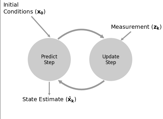
The working of a Bayesian filter is summarized in this diagram [citation needed]

\begin{flalign*} \texttt{Prediction: } \bar{\textbf{x}} = \textbf{x} * f_x(\bullet) \\ \texttt{Update: } ||{\mathcal{L}}\cdot{x}|| \end{flalign*}

1. The initialization step, as the name says, is where our belief in the state is initialized
2. The prediction step follows next. Here, the model of the system is used to estimate the value for the next system state. Any uncertainties with the belief will be accounted for here. The prediction is done by performing a convolution of a kernel function over the PDF
3. The next step is the update step. A measurement and its associated belief is taken and the likelihood is calculated based on that. the posterior is calculated using the Bayes formula

One cycle of prediction and updating with a measurement is called a system evolution

Looping the prediction step

If the sensor is noisy, we will always lose some information in the prediction. If we keep looping the prediction step on this, we will eventually end up with no information left, and the probabilities will be evenly distributed across the distribution

For most tracking and filtering applications, we want a unimodal and continuous filter. Multimodal filtering is computationally expensive and counterintuitive